In plain words
This page asks what the vacuum would have to be made of for the law to come out. The answer proposed is a glass: a crowd of tiny elements, each with a bit of slack before it pushes back, like a loose spring. Where the pull is weak, few elements are engaged and the response is soft (that is the galactic anomaly); where it is strong, all are engaged and you get Newton. Elements pushed too hard during a dense collapse never regain their slack: that is the memory. The one number that sets the scale is the expansion rate of the Universe, which fixes how cold the vacuum is. Unfamiliar words are in the glossary.
Constituents
The Hamiltonian.
A medium of identical elements, each a light mass with an elastic play and a hard core, coupled to gravity.
Element i has position ri, momentum pi, mass m, and a yield threshold qi ≥ 0 drawn from a distribution. It carries elastic stress only once the strain it feels, ui = ⟨|∇Φ|⟩/a₀ averaged over its orbit, exceeds its threshold. A hard core forbids overlap.
Nothing in this is exotic: it is the Hamiltonian of a disordered elastic medium, a glass. The physics is in three coarse-grained consequences.
Property 1 — derived, not posed
The transition function.
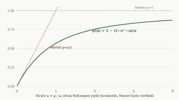
At equilibrium the mean elastic stress at strain u is σ(u) = k ⟨(u − q)+⟩ averaged over the threshold distribution. For thresholds drawn from a Boltzmann law, f(q) = e−q/q̄/q̄, a Monte-Carlo of two million elements returns, exactly,
Why the exponential, and not another distribution? Among the threshold laws that fit the SPARC rotation curves equally well, the exponential is the one of maximum entropy at fixed mean, that is, thermal equilibrium. The data do not single it out; thermodynamics does.
Property 2
Why the response is monopolar.
The medium is hot, in the sense that it carries the virial dispersion of the structure it collapsed with: 50–100 km/s in the Milky Way (a star cannot bind it at all; a dwarf galaxy's medium is correspondingly cooler). Each element samples a whole orbit before it responds. The strain it feels is the field averaged over that orbit, which for a warm population is close to the spherical mean of the enclosed mass, and carries no memory of the thin disc it passed through. A direct orbit integration in the Milky-Way potential confirms it: above about 50 km/s the orbit-averaged field loses its dependence on height above the plane. The phantom follows the smooth, hot medium, so there is no phantom disc, and the response is the spherical, monopolar law of the model.
Property 3
The memory is plastic engagement, in a glass below its transition.
Soft-glass rheology settles which phase the galactic medium is in. A glass above its noise-temperature transition (x > 1) is a fluid: it carries no stress at zero strain rate, so it could not hold a static phantom. The static law σ(u) above is that of a solid, so the medium in galaxies sits below the transition, a glassy solid with distributed slack. Memory is then not a phase change but plastic pre-strain: elements pushed past their slack during a dense collapse stay engaged (μ = 1, Newton). The hard cores make the engagement irreversible: a kinetic Monte-Carlo in the trap model of Bouchaud shows that once locked, the time to escape at the vacuum temperature is astronomically long.
This is the formation memory, and the reason the Sun sits Newtonian inside an engaged pocket. It is not an extra rule bolted on; it is the plastic behaviour of the same medium. It also has a cost: freezing releases no heat worth the name (10−53 J per element at the de Sitter temperature) but traps elastic energy, so a pocket is a metastable state of high free energy, protected kinetically, not thermodynamically.
Two components, not one
Gravitational waves cannot be the phonons of this threshold lattice. Its spacing, fixed by the Compton identity mℓ = ℏ/c and by Newton's normalisation, is 0.22 mm; a lattice that coarse would disperse gravitational waves 13 times more than GWTC-4.0 allows (ℓ < 17 µm), and any glass would damp them 1015 times more than GW170817 allows. The vacuum needs a lossless crystalline backbone carrying the waves, and on it an orientational glass carrying the slack, the memory and the MOND response: the smectic medium of the section above. See Black holes.
One input: the Hubble rate
Where a₀ comes from.
The mean threshold q̄, hence a₀, is set by the vacuum bath. An element accelerating at a feels an Unruh temperature ℏa/2πckB; the surrounding de Sitter vacuum sits at ℏH₀/2πkB ≈ 2.8×10⁻³⁰ K. The two are equal at
With a₀ fixed this way, and nothing fitted to galaxies, the law reproduces SPARC as well as a fitted MOND curve.
Classical in form, quantum in origin
Is the force quantum?
Not in the usual sense. It is the thermal, elastic response of a medium — classical in its form and its strength. The quantum part is its origin, and it hides.
The tell is that the acceleration scale carries no Planck constant. It is set by two temperatures being equal, and in that equality the ℏ’s cancel:
So the quantum content lives in the vacuum, not in the force law. It is there in two places: the medium has a temperature only because the vacuum fluctuates (the de Sitter and Unruh temperatures are both quantum-field-theory effects), and the load-bearing step of the model — that an accelerated body sees a warmer vacuum and the vacuum responds — is the Unruh effect, a property of vacuum fluctuations. The glass and its memory, by contrast, are ordinary classical statistical mechanics; they need no quantum input.
This is not quantum gravity in the usual sense. Nothing here quantizes the metric or spacetime; there is no graviton in this sector. The picture belongs to emergent, thermodynamic gravity (Sakharov, Jacobson, Verlinde, Padmanabhan): the anomalous part of gravity would be the collective thermodynamics of the vacuum’s quantum degrees of freedom, not a fundamental quantum force waiting to be quantized. And it is precisely the least settled part — asserted, following Milgrom and Verlinde, not derived. No one has closed the calculation that turns vacuum fluctuations, under acceleration, into the thermal response the model assumes.
The honest question
Is the micro-model observable?
Partly. The constituents themselves are not seen; a few of their consequences are, and they differ from plain MOND, which is what makes them worth chasing.
Distinguish two things. The ingredients — the elements, the thermal thresholds, the coupling of the vacuum to acceleration — are inferred, not observed; no instrument shows them. But the soft-glass reading makes three predictions that go beyond MOND and are, in principle, measurable:
| Micro-model feature | Observable? | How | Status |
|---|---|---|---|
| Acceleration floor: 1−μ ∝ 1/u, a constant a₀ excess at high field | Yes, indirect | Bulge-dominated and inner rotation curves; McGaugh has zero floor | SPARC hints +0.018 dex at x≈15; undecided |
| Formation memory: dense-born Newtonian, diffuse-born MOND | Yes | Wide binaries Newtonian at every separation; tidal dwarfs MOND, clusters Newtonian; kicked remnants never boosted | Gaia DR4 (Dec 2026) decisive |
| Vacuum origin of a₀: tied to Λ (constant), to H(z) (thermostat) or to the medium's density and age, (1+z)3/2 | Yes | The radial-acceleration relation at high redshift | JWST rotation curves; MUSE-DARK II and III disagree |
| Halo thickness set by the medium temperature σm | Marginal | The coldest dwarfs could keep a faint residual disc | not yet tested |
| The elements; the Unruh coupling itself | No | Inferred only; an open theoretical step | — |
The third row is the sharpest test of the microphysics as such. If a₀ comes from the asymptotic de Sitter horizon — the cosmological constant Λ — it is a true constant. If it comes from the instantaneous Hubble rate, it grows as H(z) toward the early Universe. If it comes from the density, or the age, of a medium that dilutes with the expansion, it grows as (1+z)3/2, which coincides with H(z) in the matter era and exceeds it now. The radial-acceleration relation of high-redshift galaxies separates the three.
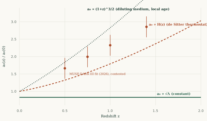
So the answer is neither “yes, we can see the glass” nor “no, it is untestable.” The medium is inferred, but its floor, its memory, and the redshift behaviour of a₀ are observable, and each could kill the picture. That is the most one can ask of an effective model whose deepest step is not yet derived.
The limits of the claim
What is not derived.
The exact coefficient in a₀ = cH₀/2π needs the real Unruh–de Sitter calculation, not a toy; the reason a vacuum element couples thermally to acceleration is the open step that Milgrom and Verlinde both leave unclosed; and the nature of the elements is not identified. This is a coherent effective model, not a first-principles theory. It also inherits MOND's failures on the ultra-faint dwarfs, clusters and the CMB.
Sources
Reproduction & references.
The calculations are Python scripts over public data: the SPARC catalogue (Lelli, McGaugh & Schombert 2016), the Gaia-based Milky Way vertical potential (2026), DiskMass (Martinsson et al. 2013), and the Solar-System bounds of Cassini (Park et al. 2026) and Mercury. Key references: Milgrom 1983 and 1999; McGaugh, Lelli & Schombert 2016; Skordis & Złośnik 2021 (relativistic completion, with tracking); Sollich 1997 and Bouchaud 1992 (soft-glass and trap models); Chae et al. 2020–2021 and Banik et al. 2024 (wide binaries and the external-field effect).
This is an exploratory research snapshot, not a peer-reviewed result. Numbers are reproducible from the scripts; the model is a working hypothesis whose decisive test is still ahead.