In plain words
Stars bob up and down through the disc of the Milky Way, and how fast they bob measures the pull toward the plane. Any modified gravity that acts on the local field predicts a thin sheet of extra pull in the plane; the Gaia measurements want a round halo instead, and the mismatch is a factor 10 to 40 in the usual goodness-of-fit. That single measurement is what rules out the whole family of local laws. The rest of this page checks that the surviving law still fits galaxy rotation and leaves the planets alone. Unfamiliar words are in the glossary.
Milky Way, vertical
No phantom disc.
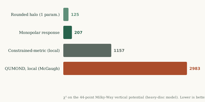
A local law builds a disc of phantom mass in the plane. The measured vertical potential wants a rounded halo.
Forty-four measurements of the vertical potential (Gaia-based, 2026) are compared to a rounded halo with one free amplitude, and to laws with none.
How to read it
The monopolar response has the halo's shape (rises as z²) with an amplitude 0.75× the fitted halo, and it predicts the local dark-matter density, 0.013 M☉/pc³, against 0.010 ± 0.003 measured. Two further data sets, DiskMass and the HI flaring of the Milky Way, agree: the phantom is a halo, not a disc.
SPARC, 147 galaxies
The rotation curves are kept.
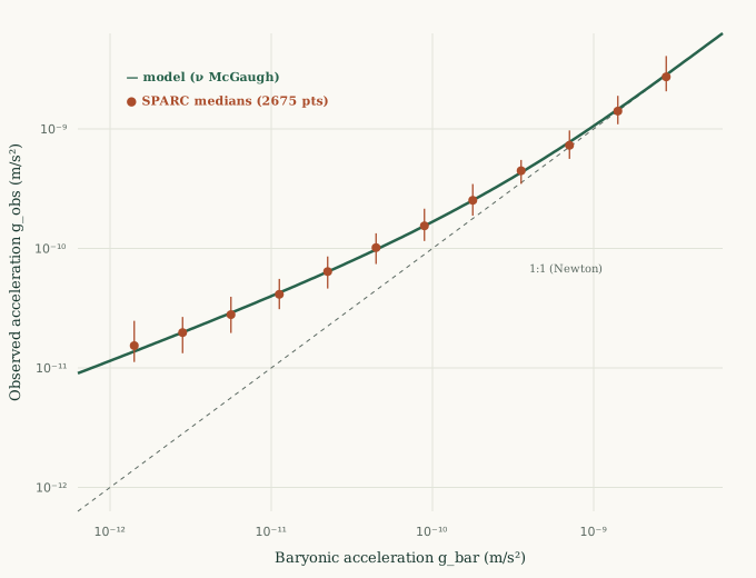
On the spherical field, the model reproduces the radial-acceleration relation with a scatter of 0.138 dex, matching a fitted MOND curve, at an acceleration scale fixed by the Hubble rate rather than fitted.
Cassini & Mercury
The Solar System is untouched, by the memory.
The transition function leaves a constant acceleration floor at high field. If the Solar medium responded, that floor would give Mercury and Saturn precessions three orders of magnitude above the measured residuals. The engaged pocket around the Sun sets the response to Newton exactly; only the smooth galactic phantom remains, and it is far below the Cassini bound.
The memory is not optional
Compatibility with Cassini and Mercury is not automatic here: it requires the pocket. The Solar System therefore tests the memory as directly as the star clusters do.
A prediction, not just a pass.
Because the Sun's pocket is fully engaged, its own field makes no phantom; only the smooth galactic-halo tide remains. That is a sharp, falsifiable claim: the outer Solar System carries no MOND quadrupole, four orders of magnitude below what a local MOND external-field effect predicts.
| Anomalous quadrupole Q₂ at Saturn | Value |
|---|---|
| This model (Sun's pocket engaged, smooth halo only) | 2.5×10⁻³¹ s−2 |
| Local MOND, with the external-field effect | 1.6×10⁻²⁷ s−2 |
| Current Cassini bound | < 3×10⁻²⁷ s−2 |
The test is clean. A tighter planetary-ranging bound that reaches 10−27 and finds a quadrupole would favour local MOND and kill this picture; continued non-detection below 10−28 kills the local MOND external-field effect instead. This model predicts Mercury and Saturn perihelia with no anomaly at any foreseeable precision.
And the Oort cloud
Newtonian throughout. The pocket has no edge inside the Oort cloud (an earlier claim of a transition near 0.15 pc is withdrawn), and the Oort peak reproduced by Newtonian simulations (Vokrouhlický et al. 2024) is a pass, not a test still to run.
Everything, at a glance
Scorecard.
- Milky-Way vertical potential (shape and amplitude)pass
- SPARC radial acceleration, 2675 points0.138 dex pass
- Acceleration scale a₀ fixed by cH₀/2πno fit pass
- Cassini quadrupole (smooth galactic phantom)2.5×10⁻³¹ s−2 pass
- Mercury perihelion, extra precession∼10−10 ″/cy pass
- Pal 14 (born dense, engaged)Newtonian pass
- Crater II dwarf~1.5–2.1 vs 2.7 km/s as MOND
- Segue 1 and the ultra-faint dwarfs15–20× too low fail
- Clusters, the Bullet, the CMBunresolved as MOND